What Is Stochastic Calculus
One of the cool things I’ve learned about in grad school is stochastic calculus. I’m far from an expert on the subject but I’m going to share the basic idea of a Stochastic Integral.
Quick Review
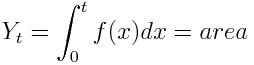
The integral everybody learns about in high school and undergrad is a Reimann Integral, where you’re finding the area under a function by partitioning the space into a sequence of rectangles. As you make the widths of the rectangles smaller, the approximation gets better, and at the limit where the rectangle widths go to zero, you get the area of the space under the curve.
Stochastic Integral
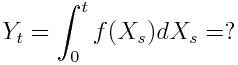
With a stochastic integral, we still partition the space into rectangles and sum up the area of the rectangles as the widths get smaller. So what makes a stochastic integral different?
Each rectangle width is a random variable!
Just think about how crazy that is, you’re now summing a series of random variables (ie. a stochastic process.) In fact, you’ll notice that the integral equation uses dXs instead of just dX like the Reimann integrals, dXs is a stochastic process that lasts for time s.
What is the output of a stochastic integral?
So a stochastic integral is a sum of widths, which are each random variables. That means the output of a stochastic integral is also a random variable. The characteristics of the random variable depend on the characteristics of the stochastic process you integrated over. The most common process to use is “Brownian Motion”/”Weiner Processes“(teehee). This describes the motion of a stock price, essentially saying it’s just as likely to go up or down at any given time. In that case the stochastic integral is a random variable that has a normal distribution, with an expected value of 0.
Why would you do this?
The first thing you might be wondering is whether this is all some elaborate homework question from a theoretical math professor. Well, the big fields which use this math are physics and finance. It’s hard to think of how to directly represent some relationship or model with a stochastic integral. However, it’s a lot easier to picture modelling some relationship with a stochastic differential equation. This would just be any value whose rate of change is dependent on the rate of change of some random process. Once you have the differential equation, you use a stochastic integral to solve for the value.
I was introduced to the concept through a finance class, so let’s look at an example from the stock market.
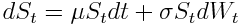
The above equation describes the price of a stock.
St is the price of the stock.
dSt is the change in the stock price.
dt is the change in time.
u is the average expected return of the stock over time.
sigma is the volatility of the stock.
dWt is the change in Brownian Motion (random ups and downs of the stock).
So the equation says that the stock price changes in relation to two terms. The first term is u * St * dt, the long term expected return of the stock times the current price of the stock times the length of time. For example, if the expected return of the stock were 3% per year (u = 0.03), and the current price of the stock was 100 (St = 100), and we wanted to the change of the stock price in one year (dt = 1) then this term would equal 3. ie. the stock price has gone up by 3 in one year. Of course stocks don’t just go up in such a predictable way, they go up and down along the way.
The second term models the random ups and downs of the stock. To be technical, the ups and downs are represented by Brownian Motion. dWt to represent the change in Brownian Motion over the time period.
Now the rate of change of the stock on its own isn’t that useful, we want to know what the actual price of the stock is at some given time (ie. solve for St.) If the dWt term wasn’t in there, you could just use basic Ordinary Differential Equation solving techniques for this. In order to deal with the change in Brownian Motion inside this equation, we’ll need to bring in the big guns: stochastic calculus, and in this case Ito’s Lemma.
Why can’t we solve this equation to predict the stock market and get rich? Remember what I said earlier, the output of a stochastic integral is a random variable. So solving this equation won’t actually give you the definite price of the stock 1 year from now, but a random variable, along with its mean and variance (assuming real world stocks actually follow Brownian Motion!)
Where can I learn more?
I learned about this through financial applications, so those are the only resources I know about. Essentially, if you carry on with more complex examples, all roads lead to the infamous Black Scholes Equation. It’s described in a fairly accessible way in the Hull book. The teacher for my financial stochastic calculus course, prof. Jaimungal at U of T also has all of his lectures and notes online. The videos are very instructive, they’re a great introduction to this field. Lecture 7 and 8 basically cover an intro to stochastic calculus independently of finance.